Every breakthrough in deep learning, from AlexNet to GPT-4, depends on one hidden component: the optimizer.
Optimizers in deep learning determine how neural networks learn, how fast they converge, and whether training succeeds at all. The evolution from SGD to AdamW is not just a sequence of algorithms; it is the story of how deep learning became scalable enough to power modern AI systems.
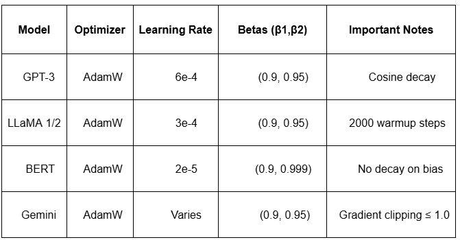
Today, nearly every major Large Language Model (LLM), including GPT, Gemini, Claude, and LLaMA, relies on AdamW during training. But reaching AdamW took more than 70 years of experimentation, mathematical insights, and engineering fixes.
The Optimizer Timeline
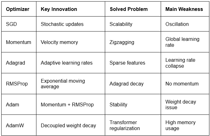
SGD (1951) → Momentum (1964) → Adagrad (2011) → RMSProp (2012) → Adam (2014) → AdamW (2017)
What Is an Optimizer?
A neural network contains millions, sometimes billions of parameters called weights. During training, the model makes predictions, compares them against real answers, and computes a loss value representing the error. The optimizer in deep learning is the algorithm responsible for updating the weights to reduce that loss.
In simple terms:
- Backpropagation computes gradients.
- The optimizer decides how to use those gradients.
- Better optimization leads to faster and more stable learning.
The fundamental update rule behind deep learning model optimization is:
\theta \leftarrow \theta – \eta \nabla_\theta L(\theta)
Where:
θ = model parameters
η = learning rate
∇L(θ) = gradient of the loss function
The optimizer’s job is essentially to move the model downhill on the loss landscape.
Also read: Tracing the Evolution: GPT-2 to GPT-OSS Architectural Deep Dive
The Foundation of Deep Learning Model Optimization
Batch Gradient Descent (~1847 / 1950s ML)
Before modern optimizers existed, machine learning relied on Batch Gradient Descent. The idea was straightforward: compute the gradient using the entire dataset before making a single parameter update
Imagine collecting feedback from 10,000 students before changing how you teach the next class. That is exactly how Batch Gradient Descent behaves.
Update rule:
\theta \leftarrow \theta – \eta \cdot \nabla_\theta L(\theta; X, y)
Why Batch Gradient Descent Was Impractical
Although mathematically stable, Batch Gradient Descent had major limitations:
- Extremely slow on large datasets
- Required loading the entire dataset into memory
- Only updated weights once per epoch
As datasets grew larger, this approach became computationally infeasible.
Strengths
- Stable gradients
- Guaranteed convergence (convex problems)
Limitations
- Very slow
- Requires a full dataset in memory
- One update per epoch
Stochastic Gradient Descent (SGD) — 1951
In 1951, Robbins and Monro introduced a breakthrough: instead of computing the exact gradient across the entire dataset, estimate it using a single random sample or mini-batch. This became known as Stochastic Gradient Descent (SGD).
Instead of waiting for an entire epoch to finish, SGD updates weights continuously during training.
Update rule:
\theta \leftarrow \theta – \eta \cdot \nabla_\theta L(\theta; x_i, y_i)
Why SGD Changed Everything
SGD solved the scalability problem that prevented neural networks from growing larger. Key improvements included:
- Frequent weight updates
- Lower memory usage
- Ability to train on massive datasets
- Mini-batch training on GPUs
Without SGD, modern deep learning would not exist.
Despite its efficiency, SGD introduced another challenge. Loss landscapes often contain narrow valleys called ravines. SGD tends to oscillate across steep directions while slowly progressing toward the minimum. This produces the characteristic zigzagging optimization path and slows convergence significantly.
Strengths
- Memory efficient
- Scales to large datasets
- Faster updates
Limitations
- Noisy gradients
- Unstable convergence
- Sensitive to learning rate tuning
PyTorch Example
					import torch
import torch.nn as nn
import torch.optim as optim

model = nn.Sequential(
   nn.Linear(784, 256),
   nn.ReLU(),
   nn.Linear(256, 10)
)

optimizer = optim.SGD(model.parameters(), lr=0.01)

for inputs, labels in dataloader:
   optimizer.zero_grad()
   outputs = model(inputs)
   loss = criterion(outputs, labels)
   loss.backward()
   optimizer.step()
Adding Memory — Momentum & Adagrad
The 1960s–2010s saw researchers borrow ideas from physics and statistics to fix SGD’s oscillation problem, and then discover an entirely new problem hiding underneath.
SGD with Momentum — 1964
The insight is pure physics: a ball rolling downhill doesn’t just respond to the current slope, but it has inertia from its past velocity. By accumulating a velocity vector across time steps, the optimizer naturally dampens oscillations and accelerates in the consistent direction of descent.
SGD treated each update in complete isolation — no memory of past gradients. Momentum gave the optimizer a sense of history. In ravine-like loss landscapes, gradients consistently point in one direction (the valley floor), so momentum accumulates and speeds up in that direction. Perpendicular oscillations cancel out because they alternate in sign. This results in faster, smoother convergence.
vₜ = β · vₜ₋₁ + (1 − β) · ∇θ L(θ)
Strengths
- Accelerates learning
- Dampens oscillation
- Works well with SGD
Limitations
- Still uses a global learning rate
- Requires tuning momentum values
PyTorch Example
					optimizer = optim.SGD(model.parameters(), lr=0.01, momentum=0.9)
optimizer_nesterov = optim.SGD(
   model.parameters(), lr=0.01, momentum=0.9, nesterov=True
)
Adagrad — 2011
Up to 2011, all optimizers used the same learning rate for every parameter. But in NLP, the word ‘the’ appears millions of times while ‘photosynthesis’ appears rarely. Should they receive the same gradient update magnitude? Absolutely not. Adagrad was the first algorithm to give each parameter its own adaptive learning rate.
Momentum improved speed but remained blind to parameter frequency. Adagrad solved the sparse feature problem: rarely-updated parameters (rare words, unusual features) get larger updates, while frequently-updated ones get smaller, more conservative updates. This was transformative for NLP and recommender systems.
Gₜ = Gₜ₋₁ + (∇θ L(θ))² // θ ← θ − (η / (√Gₜ + ε)) · ∇θ L(θ)
The Sparse Feature Problem
Rare features receive larger updates. Frequent features receive smaller, conservative updates. This made Adagrad especially effective for:
- NLP
- Sparse embeddings
- Recommendation systems
The Adagrad Dying Problem
Because Gₜ is a monotonically increasing sum of squared gradients, the effective learning rate η/√Gₜ approaches zero as training progresses — regardless of how much the loss still needs to decrease. Adagrad ‘dies’ mid-training. This critical flaw directly motivated both RMSProp and Adam.
Strengths
- Per-parameter learning rates
- Great for NLP
Limitations
- Learning rate decays toward zero
- Long training becomes ineffective
PyTorch Example
optimizer = optim.Adagrad(model.parameters(), lr=0.01)
The Adaptive Optimization Era
The next generation of optimizers in deep learning focused on solving Adagrad’s collapsing learning rate problem while preserving adaptive updates.
RMSProp — 2012
In one of the strangest publication histories in ML, Hinton introduced RMSProp not in a paper but in slide 29 of a Coursera lecture (Neural Networks for Machine Learning, Lecture 6e). It became one of the most widely cited unpublished algorithms in history.
Adagrad’s Gₜ accumulated squared gradients forever, causing the learning rate to die. RMSProp’s fix was elegant: instead of a running sum, use an exponential moving average (EMA) of squared gradients. Old gradients decay exponentially, so the learning rate is governed by recent gradient magnitudes only, but it never collapses to zero.
E[g²]ₜ = ρE[g²]ₜ₋₁ + (1−ρ)(∇θL)² // θ ← θ − η / (√E[g²]ₜ + ε)
Strengths
- Fixes Adagrad decay
- Good for RNNs
Limitations
- No momentum by default
- Early bias
PyTorch Example
optimizer = optim.RMSprop(model.parameters(), lr=0.001)
Adam — 2014
Adam stands for Adaptive Moment Estimation. Adam optimizer in deep learning combines:
- Momentum → remembers past gradients for smoother updates.
- Adaptive Learning Rates → adjusts learning rate separately for each parameter.
It is one of the most widely used optimizers in deep learning because it is fast, stable, and works well on most architectures.
θ=θ−η⋅vt+ϵmt
Where:
- mt = momentum (past gradients)
- vt = adaptive learning rate term
- η = learning rate
- ϵ = small stability value
Strengths
- Fast and stable
- Adaptive learning
- Works well across many architectures
Limitations
- Higher memory usage
- Incorrect weight decay regularization
PyTorch Example
					import torch.optim as optim
optimizer = optim.Adam(
   model.parameters(),
   lr=1e-3,
   betas=(0.9, 0.999)
)
AdamW and the Transformer Era
As transformer models became larger, researchers discovered a subtle but important issue in Adam.
The Weight Decay Problem in Adam
Traditional L2 regularization interacts poorly with Adam’s adaptive learning rates. In standard Adam:
- Weight decay becomes entangled with gradient scaling
- Different parameters receive inconsistent regularization
- Generalization performance suffers
This became a major issue for transformers and large-scale language models.
AdamW Optimizer — 2017
AdamW is an improved version of Adam that fixes the weight decay problem by separating regularization from gradient updates.
It is the standard optimizer for:
- GPT
- BERT
- LLaMA
- Gemini
θt =θt^ (Adam) − ηλθ
Where:
- λ = weight decay coefficient
- Regularization is applied separately from Adam updates
Strengths
- Proper weight decay regularization
- Stable transformer training
- Better generalization
Limitations
					import torch.optim as optim
optimizer = optim.AdamW(
   model.parameters(),
   lr=1e-4,
   weight_decay=0.01
)
Why Every LLM Use AdamW
Optimizer Comparison Summary
The Future Beyond AdamW
Although AdamW dominates modern deep learning, researchers continue exploring new optimizers for even larger models.
Emerging alternatives include:
- Lion
- Adafactor
- Sophia
- Shampoo
- Muon
Many of these aim to:
- Reduce memory usage
- Improve convergence speed
- Scale efficiently to trillion-parameter models
Optimization research remains one of the most active areas in deep learning.
The Takeaway
The journey from SGD to AdamW spans 70 years, and each step solved a specific, concrete failure mode of the previous algorithm: SGD fixed scale. Momentum fixed oscillation. Adagrad fixed sparsity. RMSProp fixed dying rates. Adam unified everything. AdamW fixed regularization. Every LLM you have ever interacted with, GPT, Gemini, Claude, and LLaMA was trained with AdamW at its core. Understanding this lineage is not just history; it is the foundation of every training decision you will make as a practitioner.
Build Scalable LLM Solutions with Xcelore
From transformer optimization to production-ready AI systems, Xcelore helps businesses build, fine-tune, and deploy Large Language Model applications at scale.
Connect with Xcelore for large language development services. Whether you need custom LLM development, RAG pipelines, AI agents, or enterprise GenAI solutions, our team can help turn AI ideas into real products. Talk to our experts.