Generative Pre-trained Transformer 2 (GPT-2) is the open-source model introduced by OpenAI, partially released in 2019 with 5 model sizes: 117, 345, 762, and 1542 million parameters. It is a decoder-only attention-based model trained on a large dataset of 8 million web pages. In simple terms, the decoder-only models are next-word prediction. This model outperforms all models before 2019. Then, in August, OpenAI released its new open-weight LLMs, gpt-oss-120b and gpt-oss-20b, its first open-weight models since GPT-2 in 2019.
In this blog, we will explore how the model evolved from GPT-2 to GPT-OSS, the design and architectural comparison between the two, and more.
Architecture Overview
GPT-2
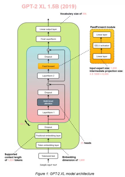
The GPT-2 model has an architecture, as you can see above, with a parameter size of 1.5 billion, the largest, along with a context length of 1024 and an embedding dimension of 1600. This GPT-2 model uses the absolute positional embeddings to keep track of the tokens in the sequence.
Besides, GPT-2 incorporated dropout layers both in its self-attention and feedforward networks to prevent overfitting on its relatively modest training corpus.
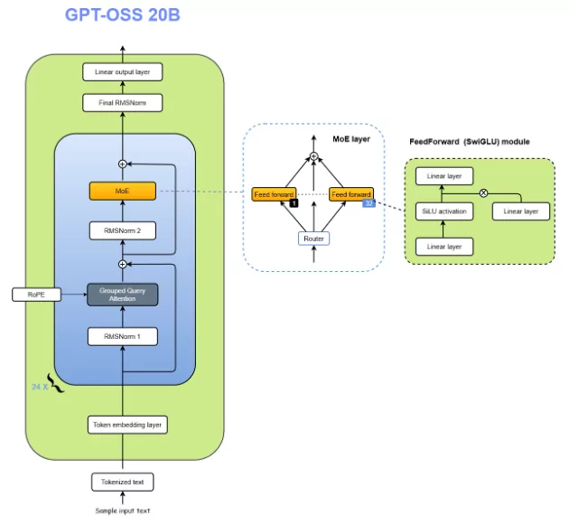
GPT-OSS 20B and GPT-OSS 120B
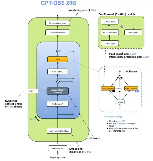
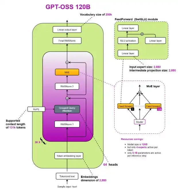
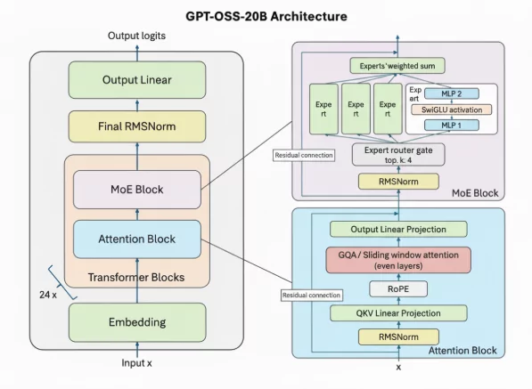
The GPT-oss models are autoregressive Mixture-of-Experts (MoE) transformers that build upon the GPT-2 and GPT-3 architectures. OpenAI has released two model sizes: gpt-oss-120b, across 36 layers (116.8B total parameters and 5.1B “active” parameters per token across 3 forward passes), and gpt-oss-20b, with 24 layers (20.9B total parameters and 3.6B active parameters per token across 3 forward passes.
The table below shows a full breakdown of the parameter counts.
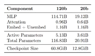
Both models have a residual stream dimension of 2880, with root-mean-square normalization applied to the activations before each attention and MoE block.
Similar to GPT-2, they use Pre-LN placement.
- Mixture-of-Experts: Each MoE block consists of a fixed number of experts (128 for gpt-oss-120b and 32 for gpt-oss-20b), along with a standard linear router projection which maps residual activations to scores for each expert. For both models, they have selected the top-4 experts for each token given by the router, and weighted each expert’s output by the softmax of the router projection over only the chosen experts. The MoE blocks use the gated SwiGLU activation function.
- Attention: Following GPT-3, attention blocks alternate between banded-window and fully dense patterns, with a bandwidth of 128 tokens. Each layer has 64 query heads of dimension 64, and uses Grouped Query Attention (GQA) with 8 key-value heads. They apply rotary position embeddings and extend the context length of dense layers to 131,072 tokens using YaRN. Each attention head has a learned bias in the denominator of the softmax, similar to off-by-one attention and attention sinks, which enables the attention mechanism to ignore certain tokens.
If you want to learn how to use these models locally, the best place to start is OpenAI’s official model hub pages:
Architecture Comparison
Now that we’ve looked at the high-level architecture from GPT-2 to GPT-OSS, let’s dive deeper into the specific components that distinguish the two models.

Now that we’ve seen the big-picture architecture of GPT-2 to GPT-OSS, it’s time to zoom in on the details. Both models are built on the Transformer backbone, but how they handle components such as positional encoding, normalization, and attention can significantly affect performance. In the section below, we’ll walk through these design choices one by one, comparing how GPT-2 approached them and how GPT-OSS takes a different (and often improved) route.
Removing Dropout
Dropout, introduced in 2012, was a widely used regularization technique designed to combat overfitting in neural networks. The idea was simple but effective for its time during training, randomly “drop out” (i.e., set to zero) a fraction of neuron activations or attention scores so that the network doesn’t rely too heavily on specific features. This forced the model to generalize better and reduced co-adaptation between neurons.
In GPT-2, dropout was retained from the original Transformer design, applied to both the attention and feed-forward layers. Back then, this made sense because most models were trained on relatively smaller datasets with multiple epochs of exposure to the same samples. In this setting, overfitting was a real concern.
However, the training dynamics of modern large language models (LLMs) are fundamentally different. Instead of looping over small datasets for hundreds of epochs, today’s LLMs are trained on massive, diverse corpora spanning trillions of tokens, often for only a single epoch, meaning each token is seen once. In this single-pass regime, the risk of overfitting is extremely low, rendering dropout largely unnecessary.
Empirical studies and replication experiments have shown that dropout not only fails to improve performance in such large-scale setups but can even slightly degrade downstream accuracy. This happens because dropout introduces noise that disrupts stable optimization in already well-regularized architectures.
Moreover, dropout adds extra computational overhead during training and inference; every layer must sample and apply random masks, which consumes both memory and time. As model sizes and sequence lengths grew, this redundant cost became more apparent.
As a result, starting from models developed after GPT-2, researchers began phasing out dropout entirely. Modern architectures omit it completely, relying instead on data scale, layer normalization, and advanced optimization techniques to ensure stable training and generalization.
This design change reflects a key shift in LLM philosophy: when data and scale act as natural regularizers, traditional techniques like dropout become obsolete. Removing it not only simplifies the model but also slightly improves efficiency and accuracy.
Rotary Positional Embeddings (RoPE) vs Absolute Positional Embeddings
Positional Embeddings are mainly applied to maintain the sequence of the input tokens.
In Absolute Positional Embeddings, the position of each token in the sentence is represented by an embedding vector of the same dimension as that of the input token, where each vector corresponds to that particular token. Then we add them together and pass them to the transformer’s inner block.
There are drawbacks to using Absolute Positional Embeddings: they only support a finite sequence length, and each positional embedding is independent of the other. In the model, positions 1 and 2 are just as different as positions 2 and 500. But the relationship in the model should be such that positions 1 and 2 are more closely related compared to position 500, which is much further away. This lack of relative positioning can hinder the model’s ability to understand the nuances of language structure.
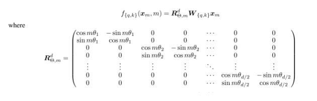
In terms of adding positional information, RoPE (Rotary Position Embedding) works differently. Instead of adding an extra position vector, it rotates the word’s vector to mark where it appears in the sentence.
Think of it like this: imagine the word “dog” as an arrow pointing in some direction. To show its position in the sentence, RoPE rotates this arrow by a certain angle. The first word might be slightly rotated, the second word a bit more, the third word even more, and so on. This method has two big advantages:
- Stability: Adding new words at the end of a sentence doesn’t shift the positions of earlier words, making it much easier to reuse past calculations (caching).
- Relative meaning: If two words (say “pig” and “dog”) always appear close together, their vectors are rotated in a way that keeps their relationship the same. This means the model remembers how words relate to each other, no matter where they appear.
General Formula for RoPE
SwiGLU vs GELU
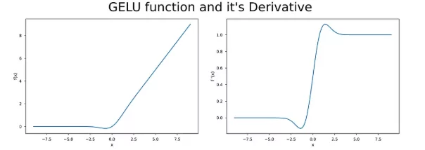
The Gaussian Error Linear Unit (GELU) is an aviation function that is a standard choice in many modern deep learning models, especially in transformer-based architectures like BERT, GPT, and T5. It is a smooth, differentiable, and non-monotonic function offering strong performance in natural language processing and other AI tasks.
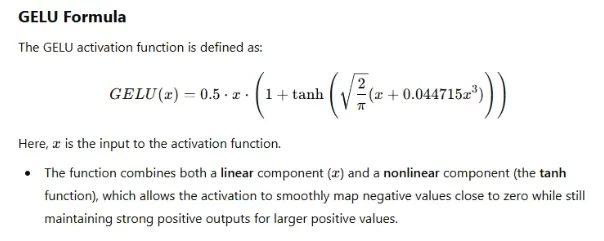
Key Characteristics of GELU
- Smooth & Differentiable: With continuous derivatives, GELU is very compatible with gradient-based optimization techniques like backpropagation.
- Non-Monotonic: Contrary to monotonic functions, GELU’s output is not always strictly increasing or decreasing with the input, thus enabling richer and more flexible learning dynamics.
- Zero-Centered: The outputs are evenly distributed around zero, which is helpful in keeping the activations balanced and reducing bias shifts during training.
- Probabilistic Nature: The nature of GELU can be interpreted as a probabilistic gating mechanism because it employs the Gaussian cumulative distribution function (CDF) to weigh inputs instead of applying a hard threshold (as done in ReLU).
Although GELU is a popular choice in large-scale models like transformers, it has certain drawbacks. The first is its computational cost. Because it depends on the Gaussian cumulative distribution function (or its approximations), it is more likely to be more resource-intensive than simpler activation functions such as ReLU. It can affect smaller setups where efficiency matters more.
Another limitation is interpretability. Unlike ReLU, GELU introduces a probabilistic formulation that can feel less intuitive, making it difficult to explain and analyze at a glance. Besides, GELU is not always the most effective option. Although it performs exceptionally well in intricate models managing enormous volumes of data, its advantages often diminish in smaller or simpler networks.
SwiGLU is an activation function that combines two powerful ideas: Swish and the Gated Linear Unit (GLU). To better understand SwiGLU, let’s first look at its building blocks.
Swish
Swish is a smooth, non-monotonic activation function, which means its output does not always increase or decrease uniformly. It is defined as:
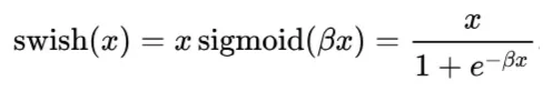
Here, β is a trainable parameter. In practice, most implementations set β = 1, which simplifies the function to: swish(x) = x * sigmoid(x)
This simplified version is often referred to as SiLU (Sigmoid Linear Unit).
One of the key advantages of Swish is that it allows smoother transitions around zero compared to ReLU. This property helps optimization and often leads to faster convergence. In fact, Swish has been shown to outperform ReLU in a variety of applications.
Gated Linear Units (GLU)
Proposed by Microsoft researchers in 2016, GLUs are designed to control the flow of information through gating mechanisms. A GLU splits the output of a linear transformation into two parts:
- One part is passed through another linear transformation.
- The other part is processed through a sigmoid activation.
The result can be expressed as:
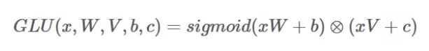
Here, the sigmoid gate decides how much of the transformed input should pass through. Much like LSTMs, these gates act as filters, allowing the network to focus on important features while suppressing irrelevant ones. GLUs have proven particularly useful in sequence modeling, machine translation, and language modeling.
SwiGLU
SwiGLU essentially replaces the sigmoid gate in GLU with the Swish function (using β=1). The formula looks like this:

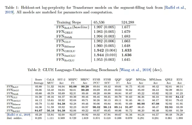
This replacement offers a more fluid and expressive gating mechanism. The SwiGLU has been applied to transformer architectures, and researchers demonstrated that it is always superior to other GLU variants in terms of log-perplexity and performance on downstream tasks.
What makes SwiGLU especially important is how it compares to GELU, the activation function used in GPT-2. GELU applies a smooth nonlinear transformation to every input, but it treats all features the same way; thus, it is not able to decide which features are of higher importance.
SwiGLU offers a learnable gate that enables the model to boost the important features selectively and, at the same time, diminish the less important ones. This not only improves representation learning but also makes the model more parameter-efficient and effective in capturing long-range dependencies.
For this reason, GPT-OSS adopts SwiGLU in place of GELU, gaining stronger performance and efficiency in large-scale language modeling.
Mixture of Experts vs Single Feedforward Module
In addition to upgrading the feed-forward module with SwiGLU (as discussed earlier), GPT-OSS takes a significant architectural leap by replacing the traditional single feed-forward block with multiple parallel feed-forward modules, collectively known as a Mixture of Experts (MoE).
This design introduces a much larger pool of parameters, as each “expert” acts like an independent feed-forward network. However, the innovation lies in how these experts are utilized. Instead of activating every expert for every token, GPT-OSS employs a router that dynamically selects only a small subset of experts to handle each token during inference or training.
This selective activation makes the system computationally sparse; only a few experts contribute to any given forward pass while maintaining a massive overall model capacity. The result is a model that can store and generalize from more knowledge (thanks to its high parameter count) without linearly increasing the computational cost.
In simpler terms, GPT-2’s single feed-forward network treats every token the same way, while GPT-OSS’s MoE mechanism enables specialization: different experts can learn to handle different linguistic or contextual patterns. This improves efficiency, scalability, and expressiveness all at once.
Fun fact: In many MoE-based large language models, over 90% of the total parameters reside in the expert networks, yet only a handful of them are used for any given token prediction.
Note: The Mixture of Experts architecture deserves a deeper exploration, so I will make a blog dedicated entirely to understanding MoE in large language models.
Grouped Query Attention vs Multi-Head Attention
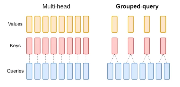
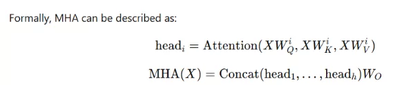
Multi-Head Attention (MHA)
Before diving into the differences, it’s worth recalling how Multi-Head Attention (MHA) works at its core. In the Transformer architecture, each token in a sequence is represented by an embedding vector. These embeddings are projected into three different spaces: Query (Q), Key (K), and Value (V), each derived using separate learned projection matrices.
In Multi-Head Attention, this process happens multiple times in parallel—one for each attention head. Each head independently learns to focus on different types of relationships within the input sequence, such as syntactic patterns, semantic associations, or positional dependencies. The outputs of all these heads are then concatenated and passed through a linear layer to form the final context representation.
While MHA is powerful and expressive, it also becomes computationally expensive as the number of heads increases. Each head maintains its own set of Key and Value projections, which multiplies both memory usage and computation. This inefficiency becomes a major bottleneck, especially in large-scale language models where attention operations are repeated thousands of times per generation.
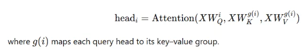
Grouped-Query Attention (GQA)
To address these limitations, Grouped-Query Attention (GQA) was introduced as a more parameter-efficient and compute-friendly alternative to traditional MHA.
The key innovation of GQA lies in sharing the Key and Value projections across multiple attention heads. Instead of every head having its own unique matrices, GQA groups several heads together and allows them to share the same Key and Value representations while maintaining independent Query projections.
For example, if a model has 4 attention heads and 2 key-value groups, heads 1 and 2 may share one set of keys and values, while heads 3 and 4 share another.
Mathematically:
This simple grouping mechanism significantly reduces memory bandwidth and lowers parameter count, since fewer key–value pairs need to be stored and retrieved during inference. In large-scale models that rely on KV caching, this optimization is especially valuable it minimizes cache size and speeds up generation without a meaningful drop in performance.
Sliding Window Attention
Sliding-window attention is an elegant optimization introduced in the Longformer (2020) paper and later refined by models like Mistral. Instead of allowing every token to attend to all previous tokens (as in standard self-attention), it restricts each token’s attention to a limited “window” of nearby tokens. This drastically reduces memory usage and computational cost a crucial improvement for scaling large models efficiently.
In gpt-oss, sliding-window attention is applied in every alternate layer. This means one layer processes the full sequence using standard Grouped Query Attention (GQA), while the next layer focuses only on a local context of 128 tokens. By alternating between global and local attention, the model maintains long-range understanding while significantly improving efficiency.
This design isn’t entirely new. GPT-3 itself used a similar idea, alternating between dense and locally banded sparse attention layers. Later models like Gemma 2 (2024) and Gemma 3 (2025) pushed this concept even further, with Gemma 3 using a 5:1 ratio of local to global attention layers.
What’s fascinating is that ablation studies from the Gemma series revealed minimal loss in model quality, even with heavy use of sliding-window attention. For gpt-oss, the choice of a small 128-token window highlights its focus on maximizing efficiency without compromising contextual understanding, a clever balance between performance and compute economy.
LayerNorm vs RMSNorm
Another subtle yet meaningful upgrade in GPT-OSS is the shift from Layer Normalization (LayerNorm), used in GPT-2, to Root Mean Square Normalization (RMSNorm). Though it might seem like a small tweak, this change represents a growing trend across modern large language models prioritizing efficiency and stability at scale.
To understand why this matters, let’s recall what normalization does. Both LayerNorm and RMSNorm serve the same purpose: they stabilize the activations within a layer, ensuring the network doesn’t diverge during training. Traditionally, BatchNorm was the go-to method for this, but it fell out of favor in transformer architectures because it struggles with small batch sizes and introduces synchronization overhead, making it less GPU-friendly.
LayerNorm works by centering (subtracting the mean) and scaling (dividing by the standard deviation) each layer’s outputs so that they have zero mean and unit variance. This is effective, but computationally expensive it requires multiple reduction operations across features.
RMSNorm, on the other hand, simplifies this process. Instead of normalizing to zero mean and unit variance, it divides the activations by their root mean square (RMS) value. This keeps the output magnitudes consistent without the need to compute mean and variance separately. In other words, RMSNorm offers similar stability benefits as LayerNorm but with fewer operations and lower communication overhead.
By removing the bias (shift) term and reducing cross-feature calculations, RMSNorm delivers faster computation and better parallelization, especially for large-scale training on GPUs. It’s a small change in theory but a smart optimization in practice, aligning with GPT-OSS’s overall design philosophy of achieving greater efficiency without sacrificing performance.
The Lasting Importance of GPT-2
Even after years of rapid progress in large language models, GPT-2 continues to hold a special place in the AI community. It stands as one of the most accessible and educational architectures for anyone looking to understand the foundations of modern transformers. While newer models like GPT-3, Mistral, or GPT-OSS are packed with optimization tricks and architectural innovations, GPT-2 remains refreshingly straightforward – a perfect balance between simplicity and sophistication.
What makes GPT-2 invaluable for learners and researchers is its clarity. It contains all the core building blocks of today’s LLMs: self-attention, positional encoding, normalization, and feed-forward layers, but without the added complexity of advanced techniques like Mixture-of-Experts, sliding-window attention, or GQA. This simplicity allows you to grasp why these later optimizations were introduced, rather than just how they work.
Starting your journey by studying or implementing GPT-2 from scratch offers deep insights into the mechanics of attention and training dynamics. Once you understand GPT-2’s design and limitations, it becomes much easier to appreciate the reasoning behind the improvements in newer models like GPT-OSS.
In essence, GPT-2 is the perfect learning ground – a gateway model that bridges the gap between foundational transformer theory and the more advanced architectures that power the AI systems of today.
At Xcelore, we specialize in advancing the frontier of AI- from architecture research to scalable LLM deployment. Whether you’re exploring open-weight model fine-tuning, custom LLM integration, or AI infrastructure optimization, our team can help you turn research into real-world performance. Connect with Xcelore to learn how we can help accelerate your AI innovation journey.
Conclusion
The journey from GPT-2 to GPT-OSS clearly shows how large language models have evolved from straightforward transformer architectures into highly optimized, large-scale intelligent systems. GPT-2 laid the foundation. It demonstrated the power of decoder-only transformers and next-word prediction at scale, making modern language AI possible. Its architecture was simple, elegant, and easy to understand—perfect for learning the fundamentals of attention, feed-forward layers, and positional encoding.
GPT-OSS, on the other hand, represents maturity in design. Instead of just increasing parameters, it focuses on efficiency and smarter computation. The model achieves significant scaling capabilities through Mixture-of-Experts, Grouped Query Attention, Rotary Positional Embeddings, RMSNorm, and sliding-window attention techniques which maintain computational expenses at controlled levels. The training methods of today which handle large datasets have been altered through the transition from GELU to SwiGLU and the elimination of dropout from training procedures.
FAQs
-
1. Can I run GPT OSS 120b locally?
Technically, yes, but it requires very high-end hardware (multiple powerful GPUs). Therefore, most users run it in the cloud or use smaller/quantized versions instead.
-
2. Can GPT-oss generate images?
No. GPT-OSS is a text-only model. While it cannot create images itself, it is highly effective at generating detailed prompts for image generation models like Stable Diffusion.